Introduction
This is where the stress energy began. In this paper, the stress spring energy is introduced and the basic idea of graph layout is to minimize it. This paper also introduce an approach to calculate the local minimization.
Spring Model
Spring energy:
$$
E=\sum_{i=1}^{n-1}\sum_{j=i+1}^n\frac{1}{2}k_{ij}(\Vert p_i-p_j\Vert -l_{ij})^2
$$
With $l_{ij}$ the desired length
$$
l_{ij}=L\times d_{ij}
$$
$d_{ij}$ is the shortest path length between node i and j.
And L can be defined as:
$$
L=L_0/\max_{i\lt j} d_{ij}
$$
$k_{ij}$ is the strength between node $i$ and $j$:
$$
k_{ij}=\frac{K}{d_{ij}^2}
$$
with $K$ a constant.
Local Minimization
The necessary condition of local minimum is:
$$
\Vert \frac{\partial E}{\partial p_m}\Vert =0\;\;\;\;for\;1\leq m\leq n
$$
In the following analysis we consider the case of 2D.
So the local minimum problem is changed to:
$$
\frac{\partial E}{\partial x_m}=\frac{\partial E}{\partial y_m}=0
$$
As the problem is not linear, what’s more, $x_i$ are not independent to each other, so another solution implemented from Newton-Raphson method is adopted.
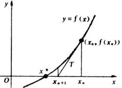
Newton-Raphson
Newton-Raphson method is an iterative way to find the solution of function:
$$
f(x)=0
$$
the method contains the following step:
- use $x_0$ as the initial point
- find the intersection of axe x and tangent of $f(x_0)$: $x_1$
- repeat step 2 at new intersections till convergence.
Solution
For node $m$:
$$
\Delta_m=\sqrt{\left(\frac{\partial E}{\partial x_m}\right)^2+\left(\frac{\partial E}{\partial y_m}\right)^2}
$$
Firstly we choose the one with maximum $\Delta_m$.
From now on we focus on axe x:
$$
\begin{aligned}
\frac{\partial E}{\partial x_i}&=\frac{\partial \sum_{j\neq i}\frac{1}{2}k_{ij}((x_i-x_j)^2+l_{ij}^2-2l_{ij}\sqrt{(x_i-x_j)^2+(y_i-y_j)^2})}{\partial x_i}\
&=\sum_{i\neq j}k_{ij}(x_i-x_j-\frac{l_{ij}(x_i-x_j)}{\sqrt{(x_i-x_j)^2+(y_i-y_j)^2}})\
&=0
\end{aligned}
$$
At the tth iteration, suppose $p_m=[x_m,y_m]$:
$$
\begin{aligned}
&\frac{\partial E/\partial x_m}{\partial p_m}(x_m(t),y_m(t))[\delta x_m,\delta y_m]\
=&[\frac{\partial^2 E}{\partial x_m^2}(x_m(t),y_m(t)),\frac{\partial^2 E}{\partial x_m\partial y_m}(x_m(t),y_m(t))]^T[\delta x_m,\delta y_m]\
=&-\frac{\partial E}{\partial x_m}(x_m(t),y_m(t))
\end{aligned}
$$
So
$$
\frac{\partial^2 E}{\partial x_m^2}(x_m(t),y_m(t))\delta x_m+\frac{\partial^2 E}{\partial x_m\partial y_m}(x_m(t),y_m(t))\delta y_m
=-\frac{\partial E}{\partial x_m}(x_m(t),y_m(t))
$$
The same as axe y, so we have two equations with two variables, and we could calculate $\delta x_m$ and $\delta y_m$, hence $[x_m(t+1),y_m(t+1)]$ is known.
After all iterations, the position of $x_m$ is optimized, so the next node m with $\max{\Delta_m}$ should be selected until
$$\max{\Delta_m}\lt\epsilon$$
Reference
[1] Kamada T. AN ALGORITHM FOR DRAWING GENERAL UNDIRECTED GRAPHS[J]. Information Processing Letters, 1989, 31(1):7-15.