Nina's Blog

Good Good Study, Day Day Up


  • Home

  • Archives

JAVA Servlet1 - thread and response head(Prime)

Posted on 2018-08-06 | Edited on 2018-09-27 | In java web , servlet

This is a realization of a simple program Prime by using java servlet.
反正就是个简单到不能更简单的实现,代码好像和书里的也没什么太大的差距。
唉这种弱智玩意儿还是打中文吧。。。

Thread in JAVA

JAVA 的 多线程编程主要流程还是放一张某博客抄来的图最简单粗暴
JAVA multi-thread programming

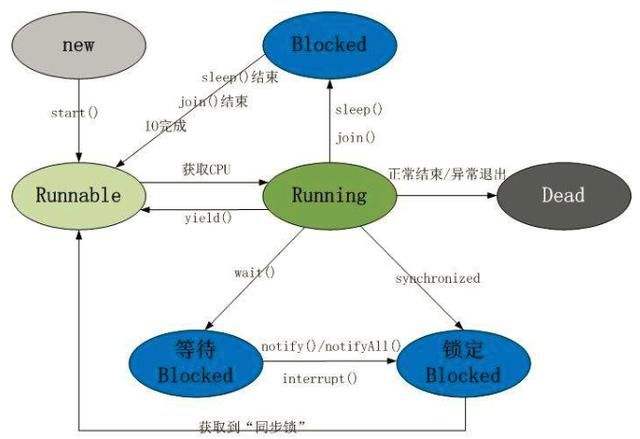
其实所有多线程编程思路都差不多,java多线程和C也没有本质上的区别(虽然C的操作系统当年就没怎么学好),这里就只简单memo一下在这份代码里用到的吧,毕竟真正的并发问题比自己随便搭个服务器玩玩要复杂太多了。

sychronized

可以适用于对象和代码上,本质就是锁住sychronized的对象,保证多线程的时候只有一个线程可以访问锁住的对象,防止了同时操作导致的各种问题。

sychronized用法主要有如下(随手写了两个有点诡异的例子):

  1. 锁住代码段:

    1
    2
    3
    public synchronized void test(){
    ...
    }

    与

    1
    2
    3
    4
    5
    public void test(){
    synchronized(this){
    ...
    }
    }

    等价。

  2. 锁住对象:

    1
    2
    3
    4
    5
    6
    7
    8
    ArrayList<int> A = new ArratList(15);
    ...
    public void test(A){
    ...
    synchronized(A){
    ...
    }
    }

注意:锁住的是同一个对象,如果在多线程操作里快乐地这么干了:

1
2
3
4
5
6
7
8
9
10
11
12
class testClass{
public synchronized void test(){
...
}
}
class myThread extends Thread {
@Override
public void run(){
testClass testC = new testClass();
testC.run();
}
}

然后在 main 里面是快乐地这么写的:

1
2
3
4
for(int i=1; i<3; i++){
Thread thread = new myThread();
thread.start();
}

那么三个线程访问的是三个testClass类里面的test函数,完全不可能被锁住。
解决方法可以加全局锁(虽然我不是很能理解为什么不选择外部创造一个全局class,或者用Runnable共享一个class),但是写代码的情况千变万化有很多情况可能上述的方法不适用。
全局锁也有两种方法:

  1. synchronized(.class):

    1
    2
    3
    4
    5
    6
    7
    8
    9
    10
    11
    12
    13
    14
       class testClass{
    public void test(){
    synchronized(testClass.class){
    ...
    }
    }
    }
    class myThread extends Thread {
    @Override
    public void run(){
    testClass testC = new testClass();
    testC.run();
    }
    }
  2. static synchronized

Runnable and Thread

又是基于个人的理解,Runnable 和 Thread 虽然从代码上来看都可以作为开启一个线程类的接口,但是从那张图来说Runnable可以理解为一个Thread准备就绪的状态,或者可以理解为,用同一个Runnable接口开启的不同线程,都是基于同一个Thread资源池来进行处理的。

Response Head

仿佛好像响应头才是书里介绍这段代码的重点,HTTP请求头和响应头的具体内容看一眼协议就行了,不想回忆我觉得我应该也没那么容易就忘了吧?吧。。。
在代码里用到的响应头是Refresh,让用户端每隔固定的时间就重新发送一次请求,也就是刷新浏览器。

1
response.setIntHeader("Refresh", 1);

整个代码的github:  Prime

用wireshark抓包的整个过程:
Prime_wireshark
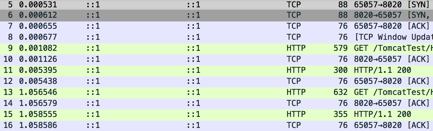
其中的什么三次握手http get就不看了,看一下第一次http response里面的内容吧

Hypertext Transfer Protocole
HTTP/1.1 200 \r\n
   Request Version: HTTP/1.1
   Status: 200
Refresh: 1\r\n
Content-Length:
Date:
…

在response包里面除了基础信息多了加粗标出来的Refresh。

ChinaVis memo

Posted on 2018-07-26 | Edited on 2018-10-11 | In visualization

Although ChinaVis is not a conference of visualization important or celebrate, there is still something interesting.

Day1: course of information theroy

Entropy

  • Shannon’s entropy:
    H(X) = -$\sum_xP(x)log(P(x))$

  • Joint entropy:
    the entropy of two events
    $H(X,Y) = -\sum_{x,y}p(x,y)log(p(x,y))$

  • Conditional entropy:
    $H(X|Y) = -\sum_{x,y}p(x,y)log(\frac{p(x,y)}{p(y)})$
    Demonstration
    $$
    \begin{aligned}
    H(X|Y) &= \sum_yp(Y=y)H(X|Y=y)\
    &= -\sum_yp(Y=y)\sum_xp(x|y)log(p(x|y))\
    &= -\sum_{x,y}p(x,y)log(p(x|y))
    \end{aligned}
    $$

  • Relative entropy (KL Divergence)
    similarity of two probability distribution
    $D_{KL}(p|q) = \sum_{x}p(x)log(\frac{p(x)}{q(x)})$

  • Mutual entropy
    Is the relative entropy of p(x,y) and p(x)p(y).
    If x and y are independent, $D_{KL}(p(x,y),p(x)p(y)) = 0$, so this indicate the dependency between X and Y.

Application Example

  1. Determine the viewpoint with least information loss.

  2. Divide the whole image into multiple blocks, using entropy to decide which block can be treated with high resolution, which with low resolution.(in order to reduce the resolution time).

Day2

Four Levels of Visualization

emmmmmmmmmmm
算了算了没什么意思

ACE:A Fast Multiscale Eigenvectors Computation for Drawing Huge Graph

Posted on 2018-07-22 | Edited on 2019-01-17 | In visualization , graph layout

Introduction

This paper[1] uses laplacian eigenmaps to calculate the coordinate of graph. However, in order to solve the running time problem in large-scale graph, the author provides an algorthm called ACE to have a fast calculation.

Background

Laplacian Eigenmaps

Given:

  • Laplace Matrix L:
    In graph G, the Laplace matrix of G: L=D-A.
    With D is the degree matrix (a diagonal matrix indicating the number of edges connected to each graph), A is the adjacent matrix.
    As described in paper[1],
    $$
    L_{ij} =
    \begin{cases}
    \sum_{k=1}^nw_{ik}& \text{i=j}\
    -w_{ij}& \text{i$\neq$j}
    \end{cases}
    $$
  • Mass Matrix M:
  • Positive Semi-Definitive Graph G(V,E,M):
    V: a set of nodes
    E: a set of weighted edges => L is positive and semi-definite.
    We can use only L and M to describe the whole graph: G(L,M)
  • A set of nodes x:
    $$x = (x_1,…,x_k,…,x_n)^T$$

Basic Idea:

Hall energy:
$$
E(x) = x^TLx = \frac{1}{2}\sum_{i,j=1}^nw_{ij}(x_i - x_j)^2
$$
target:
connected nodes should be placed near to each other.
Minimizing problem:
$$
min_x\; x^TLx
$$
with constraint which constrains the overall scale:
$$
x^TMx = 1
$$
sometimes in need of:
$$
x^TM\cdot1_n = 0
$$
to avoid the case where all the nodes are at the same location.

Solution:
Find eigenvalues that: $Lu = \mu Mu$ and choose the smallest eigenvalues.
Obviously $\mu_1=0, u_1=1_n$ is the degenerate case.
In the 2D case: $u_2$ is x-coordinate and $u_3$ is y-coordinate.

Demonstration

  1. Demonstration of Hall energy
    $$
    \begin{aligned}
    x^TLx&=x^T(D-A)x\
    &=x^TDx-x^TAx\
    &=\sum_{i=1}^n w_{ii}x_i^2-\sum_{i=1}^n\sum_{j\neq i}^nw_{ij}x_ix_j\
    &=\frac{1}{2}\sum_{i,j}w_{ij}|x_i-x_j|^2
    \end{aligned}
    $$
  2. Solution of minimization problem
    Using Lagrange Multiplier:
    $$
    f(x) = x^TLx + \lambda(x^TMx-1)
    $$
    in minimum case, derivation of f(x) is zero.
    As to the matrix derivation:
    $$
    \frac{\partial y}{\partial x} = Y\
    Y_{ij} = \frac{\partial y_i}{\partial x_j}
    $$
    so $\frac{\partial x}{\partial x} = 1_{n\times n}$
    We can calculate that:
    $$
    \begin{aligned}
    \frac{\partial f}{\partial x} &= Lx+L^Tx+\lambda Mx + \lambda M^Tx\
    &= 0
    \end{aligned}
    $$
    as L and M are symmetric matrix, so
    $$
    Lx = -\lambda Mx
    $$

ACE Algorithm

The ACE algorithm is used to accelerate the calculation of eigenvectors in large graph, such as $10^5$ node.
The algorithm is divided into two different steps, coarsening step can give us a good prediction of eigenvectors through a coarsened small graph.
The refinement step starts with the predicted eigenvectors, and use an algorithm named PI to approximate the eigenvectors to the more accurate ones.

Coarsening

The basic idea of coarsening is to project the large graph with up to $10^5$ nodes into a much smaller one.

The link between the small graph, $G^c$ here and the initial large-scale graph $G$ is the interpolation matrix $A$, which interpolates m-dimensional vectors $y \in \mathbb{R}^m$ into n-dimensional ones. The interpolation problem here is translated as:
$$x = Ay$$

Interpolation matrix

Proposition
  • A is in size of $n\times m$ with $m \lt n$
  • All elements $A_{ij} \gt 0$
  • Think A as weight, $\sum_{j=1}^mA_{ij} = 1$
  • Full column rank: Rank(A) = m
Generation
  1. Edge Contaction Interpolation
    Cluster edges into different subsets, and contract all the node in the same subset into a node.
  2. Weighted Interpolation
    //TBD

Eigenmap problem

$$min_yy^TA^TLAy\
y^TA^TMAy=1$$
with constraint
$$y^TA^TM\cdot1_n = 0$$
In order to solve this problem, we let
$$L^c = A^TLA\
M^c = A^TM$$
so the first and third problem has been changed into:
$$min_yy^TL^cy$$
and
$$y^TM^c \cdot 1_m = 0$$

Demonstration

The desmonstration here explains why we can change the problem into the laplacian eigenmap problem with $L^c$ and $M^c$.
Which means that we should prove $G^c(L^c,M^c)$ is still a semi-positive definitive graph. so
$L^c$ is semi-positive definitive
as for any x
$$
x^TLx\geq 0 \
x^TA^{T-1}L^cA^{-1}x\geq 0
$$
A diagonal and extrictly positive, so $x\neq 0 => Ax \neq 0$ is a bijection, so we can have $L^c$ is semi-positive definitive.

Moreover, since in general $M^c \neq A^TMA$, in fact, in the previous generation of the interpolation matrix, we can consider them as similar to each other.

The coarsening process can be applied further by further until we achieve a satisfying small graph.

refinement

After coarsening, we can have the eigenvectors of coarsened graph: $u_1^{‘},u_2^{‘},…,u_p^{‘}$, we can get the guessed initial eigenvectors $\hat{u_1},…,\hat{u_p}$.

Hence the refinement process refines the guessed eigenvectors to achieve an accurate eigenvectors of the initial graph.

Power Iteration Algorithm

Power iteration algorithm shows a simple approach to calculate the largest eigenvalue of a matrix.

Proposition
given a symmetric matrix A, and a non-zero normalized initial vector $v^{(0)}$, that $v^{(0)}$ is not orthogonal to the eigenvector of the largest eigenvalue. The iteration:
$$v^{(k+1)} = Av^{(k)}\v^{(k+1)} = \frac{v^{(k+1)}}{|v^{(k+1)}|}$$
converges to the largest eigenvector.

Demonstration

suppose we have a set of seperated eigenvalues
$\lambda_1,…,\lambda_n$, and the coresponding orthogonal eigenvectors $e_1,…,e_n$.

The initial vector is:
$$
v^{(0)} = c_1e_1+…+c_ne_n
$$

When multipled with matrix A k times, the vector is:
$$
\begin{aligned}
v^{(k)} &= c_1\lambda_1^ke_1 +…+c_n\lambda_n^ke_n \
&= \lambda_1^k(c_1e_1+c_2(\frac{\lambda_2^k}{\lambda_1^k})e_2+…+c_n(\frac{\lambda_n^k}{\lambda_1^k})e_n)
\end{aligned}
$$
as $\lambda_i<\lambda_1,i\gt 1$, so when k is very large, $(\frac{\lambda_i}{\lambda_1})^k\to0$

$$v^{(k)}\to\lambda_1^kc_1e_1$$
so we can calculate eigenvalue
$$\lambda_1 = \frac{v^{(k+1)}}{v^{(k)}}$$

If we normalized the vector each time:
$$
\begin{aligned}
b^{(k)} &= \frac{A^kb_0}{|A^kb_0|}\
&= (\frac{\lambda_1}{|\lambda_1|})^k\frac{c_1}{|c_1|}\frac{e_1+\frac{1}{c_1}\sum_{i=2}^nc_i(\frac{\lambda_i}{\lambda_1})^ke_i}{|e_1+\frac{1}{c_1}\sum_{i=2}^nc_i(\frac{\lambda_i}{\lambda_1})^ke_i|}\
&\xrightarrow{k\to\infty}(\frac{\lambda_1}{|\lambda_1|})^k\frac{c_1}{|c_1|}\frac{e_1}{|e_1|}
\end{aligned}
$$
Therefore, $b^{(k)}$ converges to the normalized eigenvector $e_1$.

Problem Reformulation

Let
$B=M^{-\frac{1}{2}}LM^{-\frac{1}{2}}$, $v=M^{\frac{1}{2}}u$
so the problem $Lu=\mu Mu$ is changed into:
$$
Bv=\mu v
$$
Since the power iteration algorithm can calculate the biggest eigenvalue, however, what we need is the smallest one. Therefore we reprocess $B$ into $\hat{B}$.
$$
\hat{B}=g\cdot I-B
$$
with
$$
g=max_i(B_{ii}+\sum_{j\neq i}|B_{ij}|)
$$

Demonstration

  1. $\hat{B}$ is semi-positive definitive: obvious
  2. $\hat{B}$ has the same eigenvector as $B$, but with inversed eigenvalue
    $$
    \begin{aligned}
    \hat{B}v &= g\cdot Iv - Bv\
    &= (g-\mu)v
    \end{aligned}
    $$
    So the biggest eigenvalue of $\hat{B}$ is the smallest eigenvalue of $B$. The PI can then be applied.

Algorithm

Here is the algorithm of the refinement process:

% $\hat{u_1}, \hat{u_2}, …, \hat{u_n}$ is a set of the guessed eigenvectors derived from $u_1’,u_2’,….,u_n’$
% L, M, B and $\hat{B}$ matrix already known or calculated
% $\epsilon$ is tolerance in convergence
$v_1 = M^{\frac{1}{2}}\cdot 1_n$
$v_1 = \frac{v_1}{|v_1|}$
for i = 2 to n
   $\hat{v_i}\leftarrow M^\frac{1}{2}u_i$
   $\hat{v_i} = \frac{v_i}{|v_i|}$
   repeat
       $v_i\leftarrow \hat{v_i}$
       for $j=1$ to $i-1$
          % orthogonalize to clean the part of previous calculated eigenvalues
           $v_i\leftarrow v_i-(v_i^Tv_j)v_j$
       end for
       $\hat{v_i}\leftarrow \hat{B}\cdot v_i$
       $\hat{v_i} = \frac{\hat{v_i}}{|\hat{v_i}|}$
   until $\hat{v_i}^T\cdot v_i\gt 1-\epsilon$
   $v_i\leftarrow \hat{v_i}$
   $u_i\leftarrow M^{-\frac{1}{2}}v_i$
end for
return $u_2,u_3,…,u_p$

Reference

[1] Koren Y, Carmel L, Harel D. ACE: A Fast Multiscale Eigenvectors Computation for Drawing Huge Graphs[J]. Proc IEEE Info Vis, 2002:137.

[2] K. M. Hall, ???An r-dimensional Quadratic Placement Algorithm???, Management Science 17 (1970), 219-229.

[3] En.wikipedia.org. (2018). Power iteration. [online] Available at: https://en.wikipedia.org/wiki/Power_iteration [Accessed 24 Jul. 2018].

Hello World

Posted on 2018-07-21

Welcome to Hexo! This is your very first post. Check documentation for more info. If you get any problems when using Hexo, you can find the answer in troubleshooting or you can ask me on GitHub.

Quick Start

Create a new post

1
$ hexo new "My New Post"

More info: Writing

Run server

1
$ hexo server

More info: Server

Generate static files

1
$ hexo generate

More info: Generating

Deploy to remote sites

1
$ hexo deploy

More info: Deployment

Drawing Large Graphs with a Potential-Field-Based Multilevel Algorithm

Posted on 2018-07-14

ForceAtlas2

Posted on 2018-07-06 | Edited on 2018-08-06 | In visualization , graph layout

Introduction

ForceAtlas2 是一种力导向图布局方法,设计ForceAtlas2的一个重要目的是希望能对布局变化进行连续地展现,同时让用户有一个良好的使用体验(比如收敛的时间不能过慢),另一个目的是用于进行大型网络结构的展现,所以ForceAtlas2需要适应大量的数据并且保留足够多的细节信息。

Layout Design

Energy Model

(attraction,repulstion) model

attraction,repulstion model(i.e. (a,r)-model), 已知一个layout p, 两个节点 u,v.

attraction between u,v:
$$
\omega_{(u,v)}|p_u-p_v|^a\overrightarrow{p_up_v}
$$
repulsion between u,v:
$$
\omega_u\omega_v|p_u-p_v|^r\overrightarrow{p_up_v}
$$
其中$|p_u-p_v|$指u和v的距离,在之后都用d(u,v)来表示,ω表示权值,一般情况下?$a\geq 0, r\geq 0$。

(a-r) model in ForceAtlas2

在ForceAtlas2中:a=1,r=-1.

attraction:
$$
F_a(u,v)=d(u,v)
$$
repulsion:
$$
F_r(u,v)=k_r\frac{(deg(u)+1)(deg(v)+1)}{d(u,v)}
$$
其中的阻力包含权值大小deg表示与该节点相连的边的数量。

modification of ForceAtlas2

  • LinLog mode ForceAtlas2:
    $$F_a(u,v)=log(1+d(u,v))$$
    为了对力导向图进行更好地聚类,减小了节点距离对引力的影响。
  • Gravity:
    为了防止零散的点漂走,给每个节点一个重力。
    $$F_g(n)=k_g(deg(n)+1)$$
  • Edge Weight:
    给连接u和v的边e一个重量w(e),用于修改引力:
    $$F_a(u,v)=w(e)^\delta d(u,v)$$
    w(e)由连接次数决定,用户只能通过修改$\delta$来修改w的权重
  • Dissuade Hubs mode:
    让拥有更多connection的节点作为中心节点。
    $$F_a(u,v)=\frac{d(u,v)}{deg(u)+1}$$
  • Prevent Overlapping:

    为了防止重叠,定义新的距离公式:
    $$d’(u,v)=d(u,v)-size(u)-size(v)$$
    当$d’(u,v)>0$时,用d’代替d
    当$d’(u,v)<0$时,将引力变为0,增大斥力常数$k_r$
    当$d’(u,v)=0$时,将斥力和引力都变为0

Optimization

Barnes Hut Algorithm

如果对每个点都计算其他所有节点的作用力,整个算法将变得非常复杂,计算复杂度会达到o(n2),Barnes Hut算法的主要思想就是
将距离节点n较远的一群节点看作一个节点作用于n上,方法是先将整张图用四分法分至每个叶节点里都只有一个点,再在对节点进行受力分析时判断某一正方形内的节点是否可以看作一个节点进行处理

Algorithm of quarter division of Barnes Hut

受力分析判断方法:
从根节点开始进行遍历,如果某节点的$\frac{s}{d}$值小于某阈值,其中s代表该节点的范围,d代表目标节点到该节点质心的距离,则讲这一范围内所有节点对目标节点的作用力看作一个整体,进行受力分析。详细描述见Barnes-Hut Algorithm -arborjs.

Adapting Local Speed

问题:当节点聚拢时,如果保持当前速度,很有可能在平衡状态附近震荡,而我们希望能有一张精确的力导向图,所以针对不同的节点需要有不同的速度限制。
解决方法:每个节点n被添加了一个摆动参数 $swg_{(t)}$
$$
swg_{(t)}(n)=|F_{(t)}(n)-F_{(t-1)}(n)|
$$
swg代表单位时间内n受力之差,节点的前进方向为平衡位置时n的受力差基本不变,如果节点前进方向与平衡位置相反时,需要减缓速度,我们根据swg来改变local speed s(n)
$$
s(n)=\frac{k_ss(G)}{(1+s(G)\sqrt{swg(n)})}
$$
s(G)是global speed,在下面对section中会详细说明

Adapting Global Speed

global speed 即为当前力导向图整体的速度,由两个参数 swg(G) 和 tra(G) 决定,global speed 对local speed 加以限制:
$s(n)<\frac{k_{smax}}{|F(n)|}$, $k_{smax}=10$
$$
swg(G)=\sum_n(deg(n)+1)swg(n)
$$
tra与swg相反,指代节点的前进方向为平衡位置时的受力(convergence)
$$
tra_{(t)}(n)=\frac{|F_{(t)}(n)+F_{(t)}(n+1)|}{2}
$$

$$
tra(G)=\sum_n(deg(n)+1)tra(n)
$$

$$
s(G)=\tau\frac{tra(G)}{swg(G)}
$$

Performance

与两个不同的力导向模型进行比较,发现ForceAtlas2模型在小型网络上的表现不如Yifan Hu模型,但是它
大型网络结构上有着更好地表现,它到达平衡点的速度快,并且对信息有一个更清晰的展现,ForceAtlas with LinLog Mode 可以实现更好地聚类。

Realization

github:  ForceAtlas2

Reference

[1] Jacomy M, Venturini T, Heymann S, et al. ForceAtlas2, a Continuous Graph Layout Algorithm for Handy Network Visualization Designed for the Gephi Software[J]. Plos One, 2014, 9(6):e98679.

[2] Noack A. Energy Models for Graph Clustering.[J]. Journal of Graph Algorithms & Applications, 2008, 11(2):453-480.

[3] Barnes J, Hut P (1986) A hierarchical O(NlogN) force-calculation algorithm. Nature 324:446???449

Scalable, Graph-Based Network Vulnerability Analysis

Posted on 2018-07-03 | Edited on 2018-07-05 | In Attack Graph

Introduction

This post refers to Paper “Scalable, Graph-Based Network Bulnerability Analysis”, it provides a generation method of attack graph towards specific goals。
As an complicated attack is in need of a set of exploits, and each exploit needs multiple pre-conditions and can lead to a set of post conditions. So we can find all attributes that is concerned to a goal and all the potential exploits.

Model

  • A set of attributes $A={a_1,…,a_i,…,a_n}$
  • A set of exploits $E={e_1,..,e_k,…,e_m}$
  • A set of initially satisfied attributes $ U \subset A $
  • Monotonicity: Each condition is irreversible, which means once an attributed is satisfied, it will always remain satisfied.

Classification

Each node in the graph represents an attribute and an edge means an exploit, so first of all each attribute is combined to the exploits it concerns(pre-condition and post-condition is seperated).

Secondly, classify all the attributes into different layers, the initially satisfied attributes are classified into layer 0, the number of layer means the number of exploits needed to achieve this attribute.

Now we have a classified set of attributes.

Algorithm

Algorithm of marking attributes

Analysis

Three different algorithms are proposed to find the potential paths of exploits to achieve the final goals, findMinimal, findAll and findShort.
We’ve already have:

  • A set of marked attributes and their corresponding exploits $E={e_1,..,e_k,…,e_m}$
  • A set of target attributes to be satisfied S.
    return:
  • An attack, which means a serie of exploits to meet the target att.

findMinimal

Find an attack with minimal number of exploits. (There is something can’t be understood in paper: step 3.)

findMinimal(S, att)
   $S\neq\emptyset$
     if each $s_i \in S$ is marked
       1. Choose a minimal set of expoits $E_m$ where eachs $s_i \in S$ is a post-condition of
       some $e_j \in E_m$.
       2. Prepend all the $e_j \in E_m$ to att.
       3. Select a minimal set $E’_m \subset E_m$
       4. S’ is the set of unsatisfied pre-conditions in $E’_m$.
       5. Do findMinimal(S’,att)
     endIf
   endIf

findAll

Find all potential attacks which can meet the target.

findAll(S, E$_{all}$)
   if $S \neq \emptyset$
     if each $s_i \in S$ is marked
       1. Add all exploits $E_s$ that satisfy $S$ into $E_{all}$
       2. S’ is the set of unsatisfied pre-conditions in $E_{all}$
       3. Do findAll(S’,$E_{all}$)
     endIf
   endIf

findShort

Find the shortest path (lowest level) to meet the target.

findShort(S, att)
   if $S \neq \emptyset$
     if each $s_i \in S$ is marked
       1. For each $s_i$, find $e_s$ with the smallest level n
       2. Add all $e_s$ = $E_s$ into att
       3. S’ is the set of unsatisfied pre-conditions in $E_s$.
       4. Do findShort(S’,att)
     endIf
   endIf

comment

This is a basic manual generation method, which helps generate attack graph of specific attacks and do analysis through different point of view. It provides a representative method of attack graph, which contains both advantages and disadvatages of classical attack graph method.
Users have to know all the pre and post conditions of all the exploits, and all existing attributes of all the nodes.

Reference

[1] Ammann P, Wijesekera D, Kaushik S. Scalable, graph-based network vulnerability analysis[C]// ACM Conference on Computer and Communications Security, CCS 2002, Washington, Dc, Usa, November. DBLP, 2002:217-224.

1…34
Nina

Nina

37 posts
19 categories
40 tags
© 2024 Nina
Powered by Hexo v3.9.0
|
Theme — NexT.Pisces v6.3.0